Analysis 4
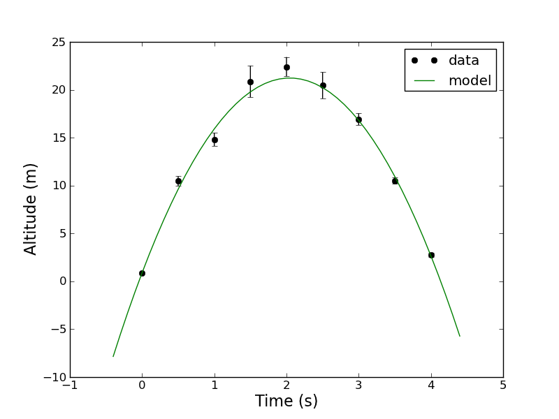
In this tutorial you will work through an example linear fit. The example is the trajectory experiment described in the previous tutorials. In this model we had altitude data <math>d_i</math> taken at times <math>t_i</math> that was modeled with a quadratic formula:
<math> d_i = a t_i^2 + b t_i + c </math>.
The following example is carried out using the python programming language. A great collection of python tools are downloadable for free (since you are students) here: [1]
Here is a file with the altitude data: media:Altitudes.txt. The first column is time and the following columns altitude data taken at the corresponding time. The multiple columns with repeated data represent repeated experiments (multiple "tosses of the projectile").
Here is the code to analyze this data (change suffix to .py) media:Linear_model.txt. The code is documented with comments (preceded by the "#" character). The code reads in the data, computes the mean and sample variance on the mean of the data at each time. It then computes the best fit, the probability to exceed as well as the variance on the model parameters.
Here is the output that you should get:
time [ 0.   0.5  1.   1.5  2.   2.5  3.   3.5  4. ]
mean [  0.8852  10.455   14.8192  20.8646  22.4106  20.465   16.9212  10.5114
   2.7726]
std on mean [ 0.04827836  0.50863592  0.68481835  1.64741573  1.01026263  1.36580654
  0.60635957  0.34929654  0.22239846]
data shape (9,)
N_inv shape (9, 9)
M shape (9, 3)
MT shape (3, 9)
a,b,c =  [ -4.86139735  19.88867809   0.88890815]
var(a,b,c) =  0.0115034026436 0.167905279208 0.00232097475846
[-0.00370815  0.83710214 -1.09698889  1.08081875  1.18992507  0.23813005
  0.11883372 -0.43576394  0.11133707]
[  1.37503988e-05   7.00739994e-01   1.20338463e+00   1.16816917e+00
   1.41592166e+00   5.67059231e-02   1.41214527e-02   1.89890215e-01
   1.23959428e-02]
[  9.32320000e-03   1.03484200e+00   1.87590470e+00   1.08559143e+01
   4.08252230e+00   7.46171000e+00   1.47068770e+00   4.88032300e-01
   1.97844300e-01]
chisq = 8.97399733731 with 6 dof
PTE =  0.175045732295
You should also obtain the following graph of the data with the model fit
