Analysis 5: Difference between revisions
| Line 38: | Line 38: | ||
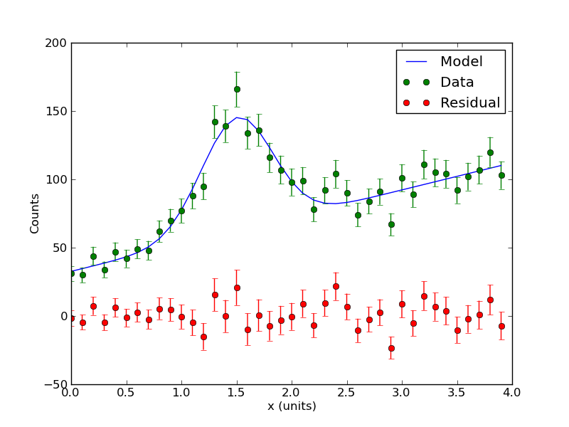
The program should also output some plots. Among them is the best fit model plotted through the data points: | The program should also output some plots. Among them is the best fit model plotted through the data points: | ||
[[ | [[file:Counts_with_fit.png]] | ||
Revision as of 01:14, 11 February 2012
In the past few tutorials, you learned how to fit data using a linear model. While many datasets may be fit with such a model, other datasets, including some that you encounter in the lab course, will not be described by linear models. Remember that a model is linear if it is linear in the parameters, so a nonlinear model must be nonlinear in the parameters. When fitting a nonlinear model, there is generally no analytic solution to the <math>\chi^2</math> minimization problem. Instead, a numerical technique is used to explore parameter space in search of the <math>\chi^2</math> minimum. A standard technique is to start at some point in parameter space and follow the gradient of the function towards the minimum, also using information about the curvature, where useful. A standard algorithm is called the Levenburg-Marquardt algorithm which uses the gradient and Hessian of the <math>\chi^2</math> to find the best fit values and their associated variance. You can learn more about this by reading the associated sections in Press, Teukolsky, Vetterling, Flannery, Numerical Recipes in C (Available online). Also you can check out the associated section in my notes from from last year media: Data_reduction_notes.pdf. Instead of diving into the details here, we provide a worked example.
The following example is carried out using the python programming language. A great collection of python tools are downloadable for free (since you are students) here: [1]
Nonlinear Model Example
Here we introduce some data <math>c_i</math> representing, say, the number of gamma-rays incident on a detector. These data are sorted by their energy <math>e_i</math>. We model the counts as a function of their energy:
<math> c_i = A \exp(-(e_i-B)^2/(2 C^2)) + Dx + E </math>
Here the parameters are the amplitude A, offset B, and width C of a Gaussian peak -- presumably modeling some emission line in the data. There is also a linear background with slope D and offset E. This example is particularly relevant to the nuclear spectroscopy lab. Because this is count data, we can use Poisson statistics to estimate the variance of the data: the variance of <math>c_i</math> is just <math>c_i</math>.
Here is the data for non-linear model and confidence interval example: media:counts.txt. The first column is energy, the second column is counts.
Here is the code (change sufixx to .py): media:Nonlinear_model.txt. The code contains comments so you follow the execution and hopefully reuse it for your own work. The code reads in the data file and fits a the nonlinear model using a Levenburg-Marquardt-based algorithm. The model determines the best fit as well as the parameter covariance matrix (and therefore the errors on the parameters). It also computes the <math>\chi^2</math> value of the best fit and evaluates the probability to exceed this value. The program should print the following values:
[ 0.   0.1  0.2  0.3  0.4  0.5  0.6  0.7  0.8  0.9  1.   1.1  1.2  1.3  1.4
  1.5  1.6  1.7  1.8  1.9  2.   2.1  2.2  2.3  2.4  2.5  2.6  2.7  2.8  2.9
  3.   3.1  3.2  3.3  3.4  3.5  3.6  3.7  3.8  3.9]
[  31.   30.   44.   34.   47.   42.   49.   48.   62.   70.   77.   88.
   95.  142.  139.  166.  134.  136.  116.  107.   98.   99.   78.   92.
  104.   90.   74.   84.   91.   67.  101.   89.  111.  105.  104.   92.
  102.  107.  120.  103.]
A= 82.7632550246 +/- 6.09661566067
B= 1.50411352295 +/- 0.0243586882858
C= -0.32584820157 +/- 0.0254629737597
D= 19.8662901184 +/- 1.16145499077
E= 32.6492609413 +/- 2.58896966419
Chi-Sq = 36.4655268717
dof =  35
PTE =  0.400407320107
The program should also output some plots. Among them is the best fit model plotted through the data points:
