Analysis 5

Back to 2012 Main Page

In the past few tutorials, you learned how to fit data using a linear model. While many datasets may be fit with such a model, other datasets, including some that you encounter in the lab course, will not be described by linear models. Remember that a model is linear if it is linear in the parameters, so a nonlinear model must be nonlinear in the parameters. When fitting a nonlinear model, there is generally no analytic solution to the <math>\chi^2</math> minimization problem. Instead, a numerical technique is used to explore parameter space in search of the <math>\chi^2</math> minimum. A standard technique is to start at some point in parameter space and follow the gradient of the function towards the minimum, also using information about the curvature, where useful. A standard algorithm is called the Levenburg-Marquardt algorithm which uses the gradient and Hessian of the <math>\chi^2</math> to find the best fit values and their associated variance. You can learn more about this by reading the associated sections in Press, Teukolsky, Vetterling, Flannery, Numerical Recipes in C (Available online). Also you can check out the associated section in my notes from from last year media: Data_reduction_notes.pdf. Instead of diving into the details here, we provide a worked example.

The following example is carried out using the python programming language. A great collection of python tools are downloadable for free (since you are students) here: [1]

Nonlinear Model Example

Here we introduce some data <math>c_i</math> representing, say, the number of gamma-rays incident on a detector. These data are sorted by their energy <math>e_i</math>. We model the counts as a function of their energy:

<math> c_i = A \exp(-(e_i-B)^2/(2 C^2)) + Dx + E </math>

Here the parameters are the amplitude A, offset B, and width C of a Gaussian peak -- presumably modeling some emission line in the data. There is also a linear background with slope D and offset E. This example is particularly relevant to the nuclear spectroscopy lab. Because this is count data, we can use Poisson statistics to estimate the variance of the data: the variance of <math>c_i</math> is just <math>c_i</math>.

Here is the data for non-linear model and confidence interval example: media:counts.txt. The first column is energy, the second column is counts.

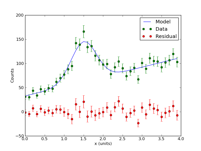
Here is the code (change sufixx to .py): media:Nonlinear_model_no_frills.txt. The code contains comments so you follow the execution and hopefully reuse it for your own work. The code reads in the data file and fits a the nonlinear model using a Levenburg-Marquardt-based algorithm. The model determines the best fit as well as the parameter covariance matrix (and therefore the errors on the parameters). It also computes the <math>\chi^2</math> value of the best fit and evaluates the probability to exceed this value. The program should print the following values:

[ 0.   0.1  0.2  0.3  0.4  0.5  0.6  0.7  0.8  0.9  1.   1.1  1.2  1.3  1.4
  1.5  1.6  1.7  1.8  1.9  2.   2.1  2.2  2.3  2.4  2.5  2.6  2.7  2.8  2.9
  3.   3.1  3.2  3.3  3.4  3.5  3.6  3.7  3.8  3.9]
[  31.   30.   44.   34.   47.   42.   49.   48.   62.   70.   77.   88.
   95.  142.  139.  166.  134.  136.  116.  107.   98.   99.   78.   92.
  104.   90.   74.   84.   91.   67.  101.   89.  111.  105.  104.   92.
  102.  107.  120.  103.]
A= 82.7632550246 +/- 6.09661566067
B= 1.50411352295 +/- 0.0243586882858
C= -0.32584820157 +/- 0.0254629737597
D= 19.8662901184 +/- 1.16145499077
E= 32.6492609413 +/- 2.58896966419
Chi-Sq = 36.4655268717
dof =  35
PTE =  0.400407320107

The program should also output some plots. Among them is the best fit model plotted through the data points (green) and the residual (red). The residual is just the data minus the model. By showing where your data deviates form the model (or vice versa), the residual is a powerful tool for diagnosing problems with your analysis.