Analysis 2

Back to 2012 Main Page

A Model for Data

From the previous analysis tutorial, you have an idea of how to estimate errors on data, including the mean of data. And you know some basic error propagation. In this tutorial, we begin the discussion of modeling data, and in particular introduce the <math>\chi^2</math> goodness of fit parameter.

So let's say you have measured <math>N</math> data <math>d_i</math> along with some estimates of the error/standard deviation <math>s_i</math>. You took these data with respect to some well determined independent variable <math>t_i</math>. As an example, you could have measured the altitude of a projectile (<math>d_i</math>) as a function of time (<math>t_i</math>). In this example you would expect the altitude of the data to be modeled by

<math> d_i = a t_i^2 + b t_i + c </math>

where <math>a, b, c</math> are model parameters corresponding to the acceleration, initial velocity, and initial displacement of the projectile. (Q: How would you have measured the error for the data? A: You could have run the experiment -- that is, tossed the projectile -- a number of times and computed the sample variance of the trials.)

<math>\chi^2</math> and Goodness of Fit

For a given set of parameters <math>a, b, c</math>, we need to evaluate how well the model fits the data -- the goodness of fit. For this purpose, you can use the <math>\chi^2</math>. You construct the <math>\chi^2</math> of the model, given the data, like so

<math> \chi^2 = \sum_i^N \frac{(d_i - (a t_i^2 + b t_i + c))^2}{s_i^2} </math>,

where we have continued to use the example model from the previous section. The numerator is the difference between our data and the model, squared and normalized by our estimate of the variance. Finding the "best fit" model in practice involves minimizing <math>\chi^2</math>.

Now let's suppose that the model does indeed apply to the phenomenon measured by the experiment and that we have chosen the right model parameters $a,b,c$. In this case <math>a t_i^2 + b t_i + c</math> is the expectation value for <math>d_i</math>. If this is the case then the expectation of the numerator of the <math>\chi^2</math> expression is

<math> \langle (d_i - (a t_i^2 + b t_i + c))^2 \rangle = \langle (d_i - \mu_{d_i})^2 \rangle = \sigma_{d_i}^2 \approx s_i^2 </math>,

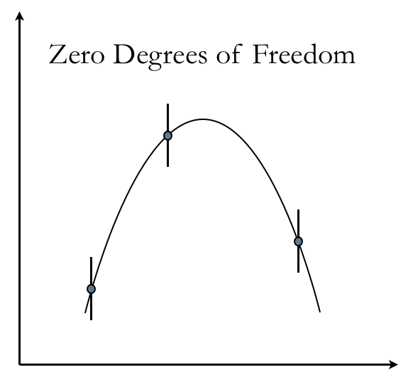
where we have used the definition of variance <math> \sigma_{d_i}^2 </math> from the previous tutorial. Given this result, the expectation value for our goodness of fit becomes <math>\langle \chi^2 \rangle = N</math>. This turns out not to be the whole story, because we don't know nature's choice of <math>a, b, c</math> and need to fit the model to the data -- more on how to do this below. If we find the best fit <math>a, b, c</math> to the data, then our expectation value for the goodness of fit is <math>\langle \chi^2 \rangle = N - 3</math>, where 3 corresponds to the number of parameters in our model, in this case <math>a, b, c</math>. More generally, if we have <math>M</math> parameters, the expectation for <math>\chi^2</math> associated with a good "best fit" model is called the number of degrees of freedom of the fit: <math>N-M</math>. To understand this, let's take the case where we have taken only three data points (<math>N=3</math>) of our trajectory. Because three points define a quadratic function, these three points determine exactly a best fit parabolic trajectory and the numerator of <math>\chi^2</math> is identically zero and therefore <math>\chi^2 = 0 = N-3</math>. Here is an example of a fit with zero degrees of freedom:

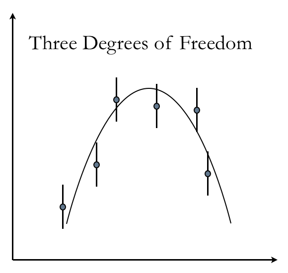
Note how the model, which is the continuous curve, goes directly through the data points, which also have error bars. When you get more data, say <math>N=6</math>, then there is no solution that results in <math>\chi^2 = 0</math>. Here is a healthy <math>N=6</math>, 3 degrees of freedom fit.

With the added data, now you can see that the <math>\chi^2</math> is non zero.

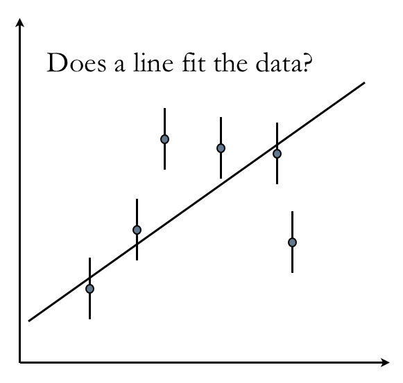
Okay, next let's consider what happens if a model does not apply to the data. Let's say we want to try to fit the trajectory data with a line. The best fit straight line for the <math>N=6</math> dataset would look something like this

(How many degrees of freedom in this fit?) Because the points have a significantly larger scatter about the best fit line than was the case for the quadratic function, the <math>\chi^2</math> will be significantly larger for this line model than it would be for the quadratic. A high <math>\chi^2</math> value -- one that is significantly larger than the number of degrees of freedom -- indicates that the model is not a good fit to the data.

Probability To Exceed

At this point, you might be wondering quantitatively about <math>\chi^2</math> and asking "how big is too big"? To answer this question, we'll introduce the concept of probability to exceed or PTE. The PTE is a function <math>\chi^2</math>. Given an input <math>\chi^2</math> and a number of degrees of freedom, the PTE function returns the probability that the experiment could have a <math>\chi^2</math> in excess of the input value. If the PTE is greater than, say, 0.05 (i.e., 5%), then you are okay -- this means that one out of twenty experiments would get a <math>\chi^2</math> larger than you found. But if the PTE is 0.01 or smaller, that means that something is wrong either with the model or your data -- it is unlikely that your experiment is rarer than one-out-of-one-hundred event.

Deriving the PTE is beyond the scope of this tutorial, but we introduce the concept because it's useful, and many libraries, including that used for the analysis examples in these tutorials, provide a PTE function.